Most climate predictions rely on output from computer models, such as those utilized by the
Intergovernmental Panel on Climate Change (IPCC).
Although predictive models are extremely useful for simulating long-term trends under different
scenarios of greenhouse gas (GHG) emissions, they do not necessarily resolve variability mechanisms
sufficiently to make reliable local and regional-scale projections, especially over decade
time scales. Climate Futures fills this gap by emphasizing plausible scenarios that can be drawn from
trends in the location-specific climate record. These scenarios can also consider climate-commodity
relationships that may exist.
The steps below provide a roadmap for developing plausible scenarios in the Climate Futures framework.
But first, you may want to familiarize yourself with the data tools on Climate Reanalyzer by visiting
the page
Explore Climate Change. Also refer to the report Coastal Maine Climate Futures, which can be used as a template to follow.
In developing plausible future climate scenarios, it is important to first define the problem and to
make an initial assessment. Identify the region of interest, plausible scenario timeframes (e.g.
2020-2030, 2030-2050) the various human and natural systems
likely to be impacted (e.g., agriculture, forest resources, water resources, local animal
habitats), and make general list of anticipated climate impacts (e.g., heat waves, drought,
changes in the growing season, extreme precipitation, sea-level rise and coastal erosion).
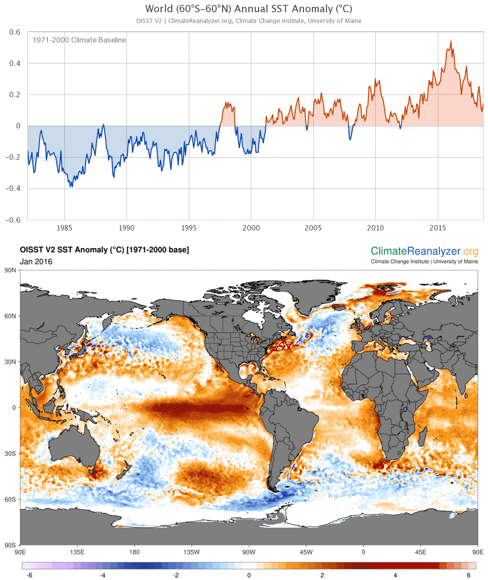
Temperature is a key climate variable, and most parts of the globe are expected to warm considerably
over the next century in response to rising GHG concentrations in the atmosphere. Thus, as part of
an initial assessment, it is useful to consider the range of future temperature outcomes projected
by global climate models (see below). These models are useful for broad-brush estimates of what is
physically possible over the next century, and they can serve as the basis for at least one plausible
scenario developed in concert with other scenarios based on trends in the historical record.
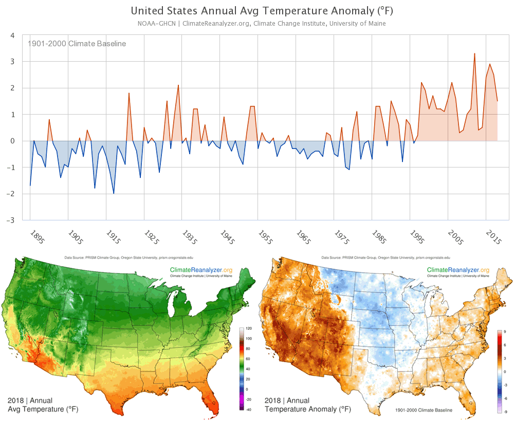
Important insights about climate change can be gleaned by taking a close look at historical records of key
meteorological variables. Examine timeseries of temperature and precipitation — annual,
seasonal, and monthly — for the location of interest. Also consider changes in the seasonal
cycle, as environmental systems are particularly sensitive to changes in the duration of the frost
and growing seasons. Note long-term trends, decadal variability, and years of extremes. This kind of
information provides important context. Perhaps some extreme years in the historical record can be
used as analogs in the future. Or perhaps the record shows surprising variability that might be
important to consider as a possible outcome over the next 10, 20, or 30 years.
Recommended data interfaces on Climate Reanalyzer:
Since at least the 1960s, changes in climate have been dominated by warming associated with
increasing concentration of greenhouse gases in the atmosphere from human activity. However, there are
sources of natural variability — for example, volcanic eruptions, solar changes, and ocean dynamics
— that will continue to influence climate. It is important to consider to what extent these
phenomena could impact your region of interest, particularly over timescales of several years.
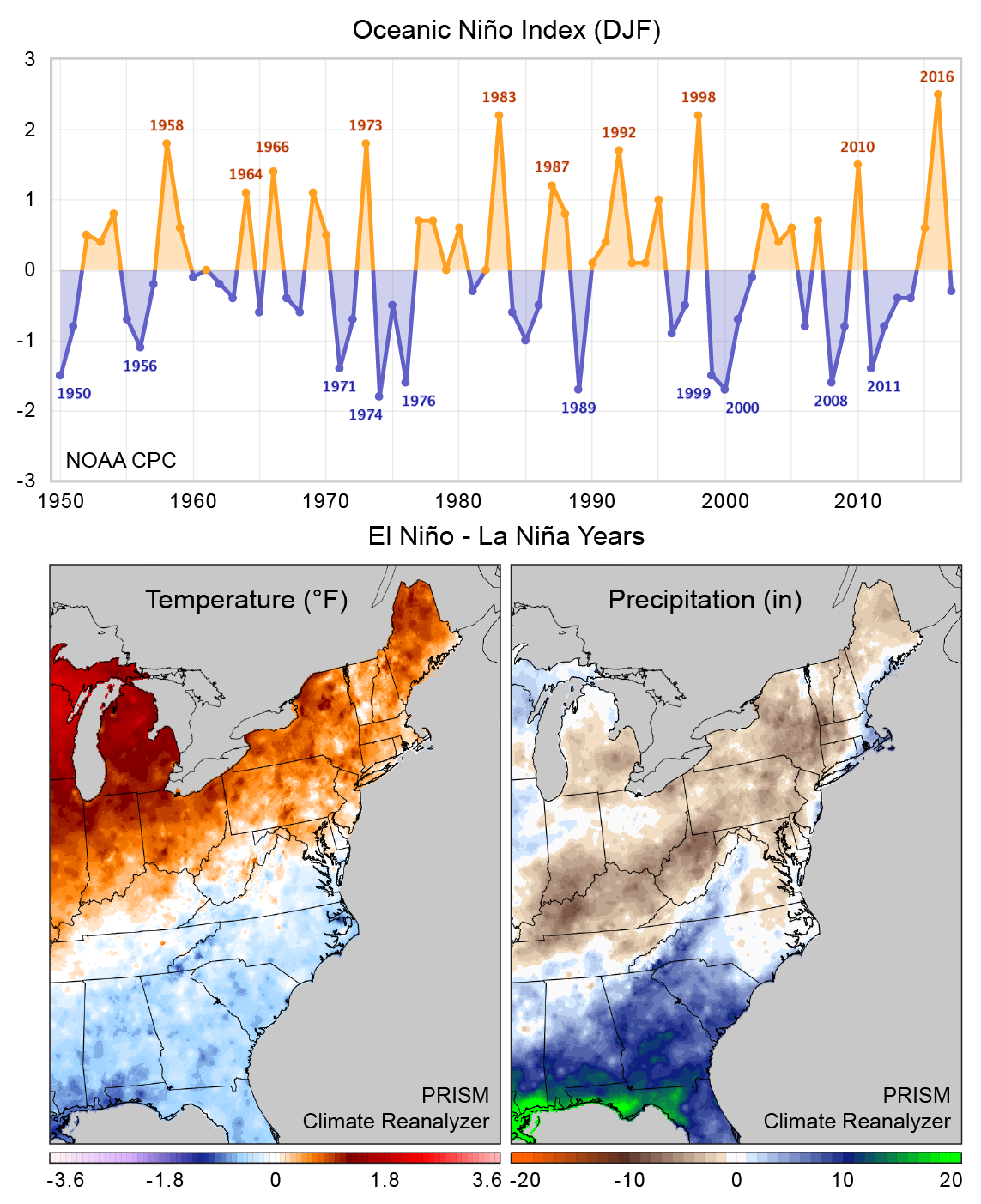
Perhaps the most prominent source of variability is the El Niño Southern Oscillation
(ENSO). ENSO is a recurring change in sea
surface temperature (SST) and atmospheric patterns across the tropical Pacific that affects global climate
on 2-7 year timescales. There are two ENSO modes that develop with differing intensities: El Niño (warm)
and La Niña (cool). The impacts of ENSO vary across the globe — some places see drought, others
more rainfall — but the regional signatures of El Niño and La Niña tend to be consistent.
Other key patterns of variability operating on a range of timescales include the Pacific
Decadal Oscillation (PDO),
Atlantic Multidecadal Oscillation
(AMO),
and North Atlantic Oscillation (NAO).
For a template that assess impacts from large-scale variability, refer to the "Climate Connections" section
in Coastal Maine Climate Futures.
Recommended data interfaces on Climate Reanalyzer:
Commodities, particularly those related to agriculture and fisheries, can be impacted by changes in
climate (e.g., as linked to changes in growing season or precipitation), and therefore it is useful
to consider climate-commodity connections in developing plausible scenario plans. Linear correlation
analysis, which measures the dependence between two random variables, can be performed for commodity
and climate timeseries. A resultant linear correlation coefficient of 1 indicates that the measured
variables exactly co-vary, whereas a linear correlation coefficient of -1 indicates that the variables
co-vary with opposite sign.
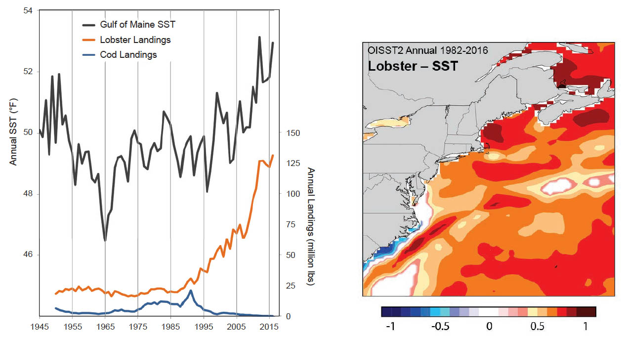
Spatial maps of linear correlation between annual commodity and climate data can be made using Climate
Reanalyzer. The figure below from
Coastal Maine Climate Futures illustrates the positive correlation between Maine annual lobster
landings and sea surface temperature (SST). In accord with findings from lobster fisheries research,
lobster abundance increases with warming ocean temperatures, at least to some threshold. An important
caution is that correlation does not necessarily mean causation — but strong correlations (> 0.5)
or anti-correlations (< -0.5) in addition to coherent spatial patterns can lend support to hypothesis,
and potentially lead to new insights.
U.S. commodity data can be readily obtained from the federal government for agriculture and fisheries.
The respective sources are the
USDA National Agriculture Statistics Service and
the NOAA Office of Science and Technology. Some commodity data are also available for
other countries from the
Organisation for Economic Co-operation and Development.
Recommended data interfaces on Climate Reanalyzer:
Plausible scenarios of future climate can be constructed once the above analyses are completed. It is
important to craft the scenarios to address all perceived areas of impact identified in the initial
assessment. Moreover, the scenarios should incorporate climate trends (e.g., summers getting warmer;
precipitation decreasing) and commodity relationships (e.g., higher crop yield may increase with
warmer summer, but decrease with more dryness) as much as possible. A decision maker may at first
be inclined to consider three outcomes or scenarios: low, medium, and high. Therefore, it is beneficial
to include at least four scenarios, with the fourth relating to perhaps an unexpected or extreme outcome
that otherwise might not be considered.
To again call upon a familiar template,
Coastal Maine Climate Futures defines five plausible scenarios in concise paragraphs as titled
below. Refer to the report document to see how the paragraphs are organized.
Climate Change Institute
University of Maine
Orono, ME 04469-5790
Tel: 207-581-2190
Fax: 207-581-1203
contactcci@umaine.edu
This work was supported by grants from the
Russell Grinnell Memorial Trust